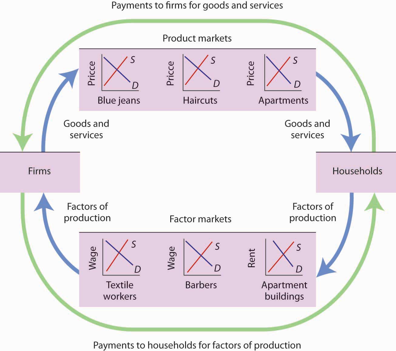
Implicit in the concepts of demand and supply is a constant interaction and adjustment that economists illustrate with the circular flow model. The circular flow model provides a look at how markets work and how they are related to each other. It shows flows of spending and income through the economy.

A great deal of economic activity can be thought of as a process of exchange between households and firms. Firms supply goods and services to households. Households buy these goods and services from firms. Households supply factors of production—labor, capital, and natural resources—that firms require. The payments firms make in exchange for these factors represent the incomes households earn.

The flow of goods and services, factors of production, and the payments they generate is illustrated in Figure 2.21 “The Circular Flow of Economic Activity”. This circular flow model of the economy shows the interaction of households and firms as they exchange goods and services and factors of production. For simplicity, the model here shows only the private domestic economy; it omits the government and foreign sectors.

Figure 2.21 The Circular Flow of Economic Activity

This simplified circular flow model shows flows of spending between households and firms through product and factor markets. The inner arrows show goods and services flowing from firms to households and factors of production flowing from households to firms. The outer flows show the payments for goods, services, and factors of production. These flows, in turn, represent millions of individual markets for products and factors of production.

The circular flow model shows that goods and services that households demand are supplied by firms in product markets. The exchange for goods and services is shown in the top half of Figure 2.21 “The Circular Flow of Economic Activity”. The bottom half of the exhibit illustrates the exchanges that take place in factor markets. factor markets are markets in which households supply factors of production—labor, capital, and natural resources—demanded by firms.

Our model is called a circular flow model because households use the income they receive from their supply of factors of production to buy goods and services from firms. Firms, in turn, use the payments they receive from households to pay for their factors of production.

The demand and supply model developed in this chapter gives us a basic tool for understanding what is happening in each of these product or factor markets and also allows us to see how these markets are interrelated. In Figure 2.21 “The Circular Flow of Economic Activity”, markets for three goods and services that households want—blue jeans, haircuts, and apartments—create demands by firms for textile workers, barbers, and apartment buildings. The equilibrium of supply and demand in each market determines the price and quantity of that item. Moreover, a change in equilibrium in one market will affect equilibrium in related markets. For example, an increase in the demand for haircuts would lead to an increase in demand for barbers. Equilibrium price and quantity could rise in both markets. For some purposes, it will be adequate to simply look at a single market, whereas at other times we will want to look at what happens in related markets as well.

In either case, the model of demand and supply is one of the most widely used tools of economic analysis. That widespread use is no accident. The model yields results that are, in fact, broadly consistent with what we observe in the marketplace. Your mastery of this model will pay big dividends in your study of economics.

What happens to the equilibrium price and the equilibrium quantity of DVD rentals if the price of movie theater tickets increases and wages paid to DVD rental store clerks increase, all other things unchanged? Be sure to show all possible scenarios, as was done in Figure 3.19 “Simultaneous Decreases in Demand and Supply”. Again, you do not need actual numbers to arrive at an answer. Just focus on the general position of the curve(s) before and after events occurred.

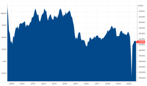
As we all know – oil is an essential input used to produce gasoline, the price of oil is a key factor that determines gasoline prices. Indeed, as statistical data show, gas prices follow oil prices very closely. The importance of oil, however, expands far beyond that. In fact, oil is used to produce nearly everything, from heating and electricity generation to plastics, fertilizers, roofing, clothing, aspirin, and guitar strings. To satisfy the demand for all those products, the world produces about 100 million barrels (3.2 billion gallons) of oil per day. No wonder that fluctuations in oil prices affect nearly all industries and may even alter the global macroeconomic situation. Because of such profound effects of oil prices on the global economy, it is important to examine the past trends in oil prices so that we could better predict how they might change in the future. And oil prices do tend to fluctuate substantially. Take a look at Figure 2.22,

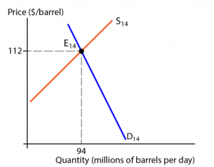
Figure 2.22 -Crude oil prices in 2012–2017

which shows how the “spot” prices of crude oil changed over the last five years. Particularly remarkable is the steep slump from about $112 per barrel to about $31 per barrel that occurred over the period from June 2014 to January 2016. It is also worthy of note that despite this 72% price drop, the consumption of oil during this period increased rather modestly: from about 94 million to about 96 million barrels per day, i.e. by only about 2%.10 What caused such a dramatic drop in the price of oil accompanied by only a slight increase in quantity? The demand and supply model discussed in this chapter will help us answer this question.

Let’s go through the four steps we’ve suggested in the previous section to help us better organize our analysis of events influencing the market for oil. First, we need to define the market we want to analyze. Since our purpose is to explain a trend in the world price of oil, not oil prices in particular countries or regions, it makes sense to examine the market for oil as a global market.11 The suppliers in this global market are all oil producers around the world, and the buyers are all world’s consumers of oil, which are predominantly businesses that use oil to produce other goods.

One important question is whether the world market for oil fits our definition of a competitive market, i.e. one where no individual seller or buyer can influence the price. Recall that the two conditions necessary for the buyers and seller to take the market price as given are (1) the product is standardized, and (2) each buyer and seller holds a very small fraction of the market, so the influence of an individual buyer or seller on the price is negligible. The first condition is certainly present, since crude oil is a standardized product (commodity). The second one does not strictly hold. The reason is that about 40% of the world’s crude oil is produced by the Organization of the Petroleum Exporting Countries (OPEC), which controls (or at least tries to) oil production in its member countries by setting production targets.

Because OPEC accounts for such a large share of the world’s market for oil, it can affect its price. Historically, crude oil prices have risen when OPEC reduced its production targets. In our demand and supply model, we can reflect this OPEC’s influence by shifting the world oil supply curve accordingly. However, OPEC’s ability to shift the world supply curve cannot change the law of supply. That is, when the price of oil rises due to OPEC’s production cuts, other oil producers have the incentive to increase their output, since it becomes more profit-able to produce more oil even if it results in higher costs. Thus, we can use the competitive demand and supply model to analyze the world market for oil. The second step is to define the initial market equilibrium. We will start from June 2014, when the equilibrium price of oil was at its peak of about $112 per barrel and its equilibrium quantity was about 94 million barrels per day.

In Figure 2.23, D14 and S14 are, respectively, the demand curve and the supply curve in June 2014, so point E14 marks the initial equilibrium. The third step is to find the new equilibrium. Note, however, that our analysis here is a little different from what we’ve done before: we al-ready know that in January 2016 the equilibrium price of oil was about $31 per barrel and the equilibrium quantity was about 96 million barrels per day. What we need to figure out is which curve shifted in which direction, as we want to explain how the market got there.

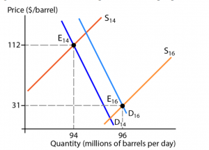
Figure 2.23 – The world market for oil, June 2014

Let’s start with the supply side. Most remarkable there is the phenomenal growth of oil production in the United States. The U.S. oil boom started in 2008, when the first well was drilled into a shale. Since then, with the help of horizontal drilling and hydraulic fracturing (commonly known as fracking), billions of additional barrels of oil have been produced. Between 2008 and 2015, U.S. oil production almost doubled, reaching 9.4 million barrels per day and threatening to surpass Saudi Arabia as the world’s largest producer of oil. In this situation, the OPEC countries faced a tough choice: cut their oil production to prop up the price, as they’ve done in the past, or maintain their output and let the price continue to fall with the purpose of driving the producers of the more costly shale oil—in the United States and everywhere else—out of business. Quite surprisingly, OPEC, led by Saudi Arabia, decided not just to go with the latter choice, but increase their oil production substantially in the hope to win the global battle for market share. The U.S. shale oil producers, however, did not back off. Armed with new drilling and other cost saving technologies, they continued to pump oil at near-record levels.

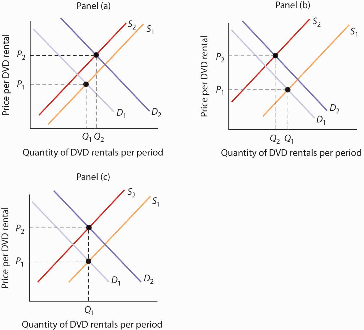
Figure 2.24 – The fall in the price of oil explained

The result was a large rightward shift of the supply curve in the world market for oil as shown in Figure 2.24, where S16 is the supply curve in January 2016. But what happened on the buyers’ side of the market? Because, as we noted earlier, oil is used to produce nearly every product, the demand for it is largely driven by the demand for all those products, which increases when economies are growing. From this perspective, although the global demand for oil increased, driven mainly by continuing economic growth in India and China, the increase was rather modest. China’s growth was shaky, and in Europe and the United States the annual rates of growth were below 3%. Thus, although the world’s demand curve for oil shifted rightward (from D14 to D16 in Figure 2.24), the effect of the demand shift was much smaller than that of the supply shift.

As you can see in Figure 2.24, since the downward effect on the price of the increased supply was much greater than the upward effect on it of the increased demand, the price dropped dramatically, from $112 per barrel in the June 2014 equilibrium (E14) to $31 per barrel in the January 2016 equilibrium (E16).

You might be wondering, however, why such a substantial drop in the price of oil resulted in only a relatively small increase in its quantity. Given that the rightward shifts of both supply and demand curves worked in the same direction, reinforcing each other to increase the equilibrium quantity, wouldn’t we expect a much greater quantity increase? The answer to the this question is that, first, the shift in the demand curve was rather small. Second, along the new same demand curve (D16) the responsiveness of the quantity of oil demanded to a change in price was very small. Economists call it a very price inelastic demand. We discuss the economic concept of the price elasticity of demand and the reasons why the demand for oil is very price inelastic in Chapter 3.

Source: Ogloblin, Constantin; Brown, John; King, John; and Levernier, William, “Microeconomics for Business” (2018). Business Administration, Management, and Economics Open Textbooks. 6.

An increase in the price of movie theater tickets (a substitute for DVD rentals) will cause the demand curve for DVD rentals to shift to the right. An increase in the wages paid to DVD rental store clerks (an increase in the cost of a factor of production) shifts the supply curve to the left. Each event taken separately causes equilibrium price to rise. Whether equilibrium quantity will be higher or lower depends on which curve shifted more.

If the demand curve shifted more, then the equilibrium quantity of DVD rentals will rise [Panel (a)].

If the supply curve shifted more, then the equilibrium quantity of DVD rentals will fall [Panel (b)].

If the curves shifted by the same amount, then the equilibrium quantity of DVD rentals would not change [Panel (c)].

Figure 2.25